Inspired by a talk N.J.Wildberger gave at our university, I expanded the Euler file for geometry. In his book "Divine Proportions", Wildberger proposes to replace the classical notions of distance and angle by quadrance and spread. Using these, it is indeed possible to avoid trigonometric functions in many examples, and to stay "rational".
In the following, I introduce the concepts, and solve a few problems. I am using symbolic computations Maxima here, which hides the main advantage of rational trigonometry that the computations can be performed by paper and pencil only. You are invited to check the results without a computer.
The point is that symbolic rational computations often yield simple results. In contrast, classical trigonometry yields complicated trigonometric results, which evaluate to numerical approximations only.
>load geometry;
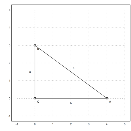
For a first introduction, we use the rectangular triangle with the famous Egyptian proportions 3, 4 and 5. The following commands are Euler commands to plot plane geometry contained in the Euler file "geometry.e".
>C&:=[0,0]; A&:=[4,0]; B&:=[0,3]; ...
 setPlotRange(-1,5,-1,5); ...
 plotPoint(A,"A"); plotPoint(B,"B"); plotPoint(C,"C"); ...
 plotSegment(B,A,"c"); plotSegment(A,C,"b"); plotSegment(C,B,"a"); ...
 insimg(30);

Of course,
![]()
where wa is the angle at A. The usual way to compute this angle, is to take the inverse of the sine function. The result is an undigestible angle, which can only be printed approximately.
>wa := arcsin(3/5); degprint(wa)
36°52'11.63''
Rational trigonometry tries to avoid this.
The first notion of rational trigonometry is a quadrance, which replaces the distance. In fact, it is just the distance squared. In the following, a, b, and c denote the quadrances of the sides.
The Pythogoras theorem simply becomes a+b=c then.
>a &= 3^2; b &= 4^2; c &= 5^2; &a+b=c
25 = 25
The second notion of rational trigonometry is the spread. The spread measures the opening between lines. It is 0, if the lines are parallel, and 1, if the lines are rectangular. It is the square of the sine of the angle between the two lines.
The spread of the lines AB and AC in the image above is defined as
![]()
where a and c are the quadrances of any rectangular triangle with one corner in A.
>sa &= a/c
                                  9
                                  --
                                  25
This is easier to compute than the angle, of course. But you lose the property that angles can be added easily.
Of course, we can convert our approximate value for the angle wa to a sprad, and print it as a fraction.
>fracprint(sin(wa)^2)
9/25
The cosine law of classical trgonometry translates into the following "cross law".
![]()
Here a, b, and c are quadrances of the sides of a triangle, and sa is the spread of at the corner A. The side a is, as usual, opposite to the corner A.
These laws are implemented in the geometry file we loaded into Euler.
>&crosslaw(aa,bb,cc,saa)
                               2
                 (cc + bb - aa)  = 4 bb cc (1 - saa)
In our case we get
>&crosslaw(a,b,c,sa)
1024 = 1024
Let us use this crosslaw to find the spread at A. To do this, we produce the crosslaw for the quadrances a, b, and c, and solve it for the unknown spread sa.
You can do this by hand easily, but I use Maxima. Of course, we get the result, we already had.
>&crosslaw(a,b,c,x), &solve(%,x)
                         1024 = 1600 (1 - x)


                                    9
                               [x = --]
                                    25
We know this already. The definition of the spread is a special case of the crosslaw.
We can also solve this for general a,b,c. The result is a formula which computes the spread of an angle of a triangle given the quadrances of the three sides.
>&solve(crosslaw(aa,bb,cc,x),x)
                 2                          2               2
             - cc  - (- 2 bb - 2 aa) cc - bb  + 2 aa bb - aa
        [x = ------------------------------------------------]
                                 4 bb cc
We could make a function of the result. Such a function is already defined in the geometry file of Euler.
>&spread(a,b,c)
                                  9
                                  --
                                  25
As an example, we can use it to compute the angle of a triangle with sides
![]()
The result is rational, which is not so easy to get if we use classical trigonometry.
>&spread(a,a,4*a/7)
                                  6
                                  -
                                  7
This is the angle in degrees.
>degprint(arcsin(sqrt(6/7)))
67°47'32.44''
Now, let us try a more advanced example.
We set three corners of a triangle as follows.
>A&:=[1,2]; B&:=[4,3]; C&:=[0,4]; ...
 setPlotRange(-1,5,1,7); ...
 plotPoint(A,"A"); plotPoint(B,"B"); plotPoint(C,"C"); ...
 plotSegment(B,A,"c"); plotSegment(A,C,"b"); plotSegment(C,B,"a"); ...
 insimg;
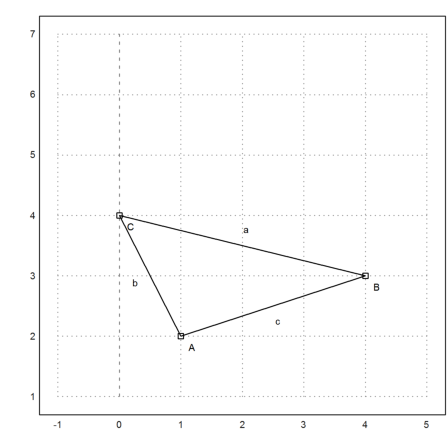
Using Pythogoras, it is easy to compute the distance between two points. I first use the function distance of the Euler file for geometry. The function distance uses classical geometry.
>&distance(A,B)
sqrt(10)
Euler does also contain functions for the quadrance between two points.
In the following example, since c+b is not a, the triangle is not rectangular.
>c &= quad(A,B), b &= quad(A,C), a &= quad(B,C),
                                  10


                                  5


                                  17
First, let us compute the traditional angle. The function computeAngle uses the usual method based on the dot product of two vectors. The result is some floating point approximation.
>wb &= computeAngle(A,B,C), &(wb/pi*180)()
                                   11
                       acos(-----------------)
                            sqrt(10) sqrt(17)

32.4711922908
Using pencil and paper, we can do the same with the cross law. We insert the quadrances a, b, and c into the cross law and solve for x.
>&crosslaw(a,b,c,x), &solve(%,x),
                           4 = 200 (1 - x)


                                    49
                               [x = --]
                                    50
That is, what the function spread defined in "geometry.e" does.
>sb &= spread(b,a,c)
                                 49
                                 ---
                                 170
Maxima gets the same result using ordinary trigonometry, if we force it. It does resolve the sin(arccos(...)) term to a fractional result. Most students could not do this.
>&sin(computeAngle(A,B,C))^2
                                 49
                                 ---
                                 170
Once, we have the spread at B, we can compute the height ha on the side a. Remember that
![]()
by definition.
>ha &= c*sb
                                  49
                                  --
                                  17
The following image has been produced with the geometry program C.a.R., which can draw quadrances and spreads.
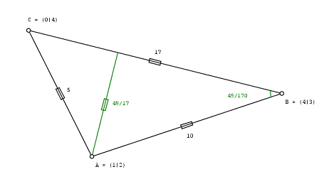
By definition the length of ha is the square root of its quadrance.
>&sqrt(ha)
                                  7
                               --------
                               sqrt(17)
Now we can compute the area of the triangle. Do not forget, that we are dealing with quadrances!
>&sqrt(ha)*sqrt(a)/2
                                  7
                                  -
                                  2
The usual determinant formula yields the same result.
>&areaTriangle(B,A,C)
                                  7
                                  -
                                  2
Now, let us solve this problem in general!
>&remvalue(a,b,c,sb,ha);
We first compute the spread at B for a triangle with sides a, b, and c. Then we compute the area squared (the "quadrea"?), factor it with Maxima, and we get the famous formula of Heron.
Admittedly, this is tough to do with pencil and paper.
>&spread(b^2,c^2,a^2), &factor(%*c^2*a^2/4)
               4         2      2   2    4      2  2    4
            - c  - (- 2 b  - 2 a ) c  - b  + 2 a  b  - a
            ---------------------------------------------
                                  2  2
                               4 a  c


          (- c + b + a) (c - b + a) (c + b - a) (c + b + a)
          -------------------------------------------------
                                 16
The disadvantage of spreads is that they do no longer simply add like angles.
However, the three spreads of a triangle satisfy the following "triple spread" rule.
>&remvalue(sa,sb,sc); &triplespread(sa,sb,sc)
                        2        2     2     2
          (sc + sb + sa)  = 2 (sc  + sb  + sa ) + 4 sa sb sc
This rule is valid for any three angles that add to 180°.
![]()
Since the spreads of
![]()
are equal, the triple spread rule is also true, if
![]()
Since the spread of the negative angle is the same, the triple spread rule also holds, if
![]()
For example, we can compute the spread of the 60° angle. It is 3/4. The equations have a second solution, however, where all spreads are 0.
>&solve(triplespread(x,x,x),x)
                                 3
                            [x = -, x = 0]
                                 4
The spread of 90° is obviously 1. If two angles add to 90°, their spread solves the triple spread equation with a,b,1. By the following computation we get a+b=1.
>&triplespread(x,y,1), &solve(%,x)
                           2       2    2
                (y + x + 1)  = 2 (y  + x  + 1) + 4 x y


                             [x = 1 - y]
Since the spread of 180°-t is the same as the spread of t, the triple spread formula also holds, if one angle is the sum or difference of the two other angles.
So we can find the spread of the doubled angle. Note that there are two solutions again. We make this a function.
>&solve(triplespread(a,a,x),x), function doublespread(a) &= factor(rhs(%[1]))
                                     2
                       [x = 4 a - 4 a , x = 0]


                            - 4 (a - 1) a
This is the situation, we already know.
>C&:=[0,0]; A&:=[4,0]; B&:=[0,3]; ...
 setPlotRange(-1,5,-1,5); ...
 plotPoint(A,"A"); plotPoint(B,"B"); plotPoint(C,"C"); ...
 plotSegment(B,A,"c"); plotSegment(A,C,"b"); plotSegment(C,B,"a"); ...
 insimg;
Let us compute the length of the angle bisector at A. But we want to solve that for general a,b,c.
>&remvalue(a,b,c);
So we first compute the spread of the bisected angle at A, using the triple spread formula.
The problem with this formula shows up again. It has two solutions. We have to pick the correct one. The other solution refers to the bisected angle 180°-wa.
>&triplespread(x,x,a/(a+b)), &solve(%,x), sa2 &= rhs(%[1])
                                           2            2
                     a   2         2      a        4 a x
            (2 x + -----)  = 2 (2 x  + --------) + ------
                   b + a                      2    b + a
                                       (b + a)


                     2                           2
             - sqrt(b  + a b) + b + a      sqrt(b  + a b) + b + a
        [x = ------------------------, x = ----------------------]
                    2 b + 2 a                    2 b + 2 a


                               2
                       - sqrt(b  + a b) + b + a
                       ------------------------
                              2 b + 2 a
Let us check for the Egyptian rectangle.
>&sa2 with [a=3^2,b=4^2]
                                  1
                                  --
                                  10
We can print the angle in Euler, after transferring the spread to radians.
>wa2 := arcsin(sqrt(1/10)); degprint(wa2)
18°26'5.82''
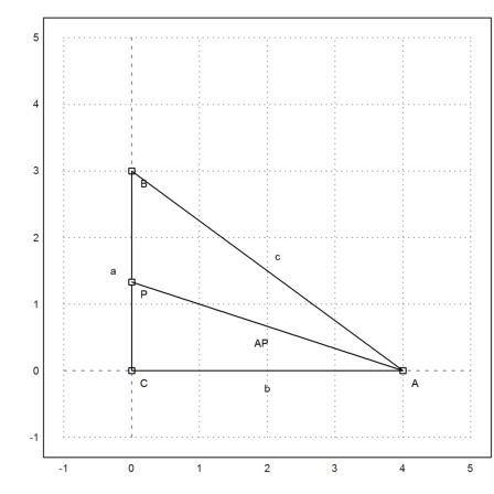
The point P is the intersection of the angle bisector with the y-axis.
>P := [0,tan(wa2)*4]
[0, 1.33333]
>plotPoint(P,"P"); plotSegment(A,P):
Let us check the angles in our specific example.
>computeAngle(C,A,P), computeAngle(P,A,B)
0.321750554397
0.321750554397
Now we compute the length of the bisector AP.
We use the sine theorem in the triangle APC. This theorem states that
![]()
holds in any triangle. Square it, it translates into the so-called "spread law"
![]()
where a,b,c denote qudrances.
Since the spread CPA is 1-sa2, we get from it bisa/1=b/(1-sa2) and can compute bisa (quadrance of the angle bisector).
>&factor(ratsimp(b/(1-sa2))); bisa &= %
                             2 b (b + a)
                       -----------------------
                       sqrt(b (b + a)) + b + a
Let us check this formula for our Egyptian values.
>sqrt(mxmeval("at(bisa,[a=3^2,b=4^2])")), distance(A,P)
4.21637021356
4.21637021356
We can also compute P using the spread formula.
>py&=factor(ratsimp(sa2*bisa))
                      b (sqrt(b (b + a)) - b - a)
                    - ---------------------------
                        sqrt(b (b + a)) + b + a
The value is the same we got with trigonometric formulas.
>sqrt(mxmeval("at(py,[a=3^2,b=4^2])"))
1.33333333333
Have a look at the following situation.
>setPlotRange(1.2); ...
 color(1); plotCircle(circleWithCenter([0,0],1)); ...
 A:=[cos(1),sin(1)]; B:=[cos(2),sin(2)]; C:=[cos(6),sin(6)]; ...
 plotPoint(A,"A"); plotPoint(B,"B"); plotPoint(C,"C"); ...
 color(3); plotSegment(A,B,"c"); plotSegment(A,C,"b"); plotSegment(C,B,"a"); ...
 color(1); O:=[0,0];  plotPoint(O,"0"); ...
 plotSegment(A,O); plotSegment(B,O); plotSegment(C,O,"r"); ...
 insimg;
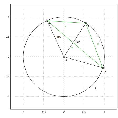
We can use Maxima to solve the triple spread formula for the angles at the center O for r. Thus we get a formula for the quadratic radius of the pericircle in terms of quadrances of the sides.
This time, Maxima produces some complex zeros, which we ignore.
>rabc &= rhs(solve(triplespread(spread(b,r,r),spread(a,r,r),spread(c,r,r)),r)[4])
                                 a b c
               - --------------------------------------
                  2                              2    2
                 c  - 2 b c + a (- 2 c - 2 b) + b  + a
We can make that an Euler function.
>function periradius(a,b,c) &= rabc;
Let us check the result for our points A,B,C.
>a:=quadrance(B,C); b:=quadrance(A,C); c:=quadrance(A,B);
The radius is indeed 1.
>periradius(a,b,c)
1
The fact is, that the spread CBA depends only on b and c. This is the chord angle theorem.
>&spread(b,a,c)*rabc | ratsimp
                                  b
                                  -
                                  4
In fact the spread is b/(4r), and we see that the chord angle of the chord b is half the center angle.
>&doublespread(b/(4*r))-spread(b,r,r) | ratsimp
0